ChainerでDeep learning入門 多層パーセプトロンで分類問題を解く
食わず嫌いだった,Deep Learningに入門してみようと思う. なんとなくChainerを使おうと思う. 今回は,使い方を覚える意味で,多層パーセプトロン (Multi Layer Perceptron, MLP) を扱ってみる. タスクは分類で,線形分離不可なデータの代表例である,XORをデータとして用いる. XORは↓みたいな形をしている.
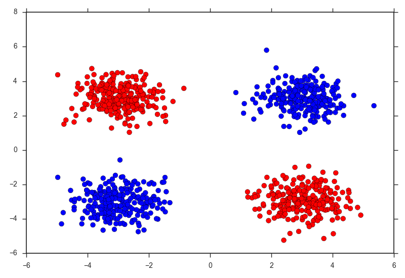
これは以下のようにして生成できる.
def make_xor(n, random_state=1, scale=3.0):
    n1, n2 = int(n/4), int(n/4)
    r = np.random.RandomState(random_state)
    X = np.r_[r.multivariate_normal([-scale,scale],[[0.5,0.0],[0.0,0.5]],n1),
              r.multivariate_normal([scale,scale],[[0.5,0.0],[0.0,0.5]],n2),
              r.multivariate_normal([scale,-scale],[[0.5,0.0],[0.0,0.5]],n1),
              r.multivariate_normal([-scale,-scale],[[0.5,0.0],[0.0,0.5]],n2)]
    y = np.concatenate([np.repeat(0,n1),np.repeat(1,n1),np.repeat(0,n1),np.repeat(1,n1)])
    return np.float32(X), np.int32(y)
chainerではfloat32, int32しか扱えないため,最後に型を変更している.
さて,多層パーセプトロンをchainerを使って実装していく. chainerを使えば,様々なニューラルネットが本当に簡単に実装できる. 多層パーセプトロンは以下のように実装できる.
class MLP(Chain):
    def __init__(self, n_out, n_units=500):
        super(MLP, self).__init__(
            l1=L.Linear(None, n_units),  # n_in -> n_units
            l2=L.Linear(None, n_units),  # n_units -> n_units
            l3=L.Linear(None, n_out),    # n_units -> n_out
        )

    def __call__(self, x):
        h1 = F.relu(self.l1(x))
        h2 = F.relu(self.l2(h1))
        y = self.l3(h2)
        return y
これは,入力も含めて3層からなるネットワークであり,以下のように式で表せる.
コード中で,出力層の活性化関数にソフトマックス関数ではなく,恒等写像を用いているのは,損失関数に交差エントロピーを用いるためである. これは,このモデルを食わせるClassifier内部に実装がある (Tutorial抜粋).
class Classifier(Chain):
    def __init__(self, predictor):
        super(Classifier, self).__init__(predictor=predictor)

    def __call__(self, x, t):
        y = self.predictor(x)
        loss = F.softmax_cross_entropy(y, t)
        accuracy = F.accuracy(y, t)
        report({'loss': loss, 'accuracy': accuracy}, self)
        return loss
実際に学習させていきます. extensionsを使えば,損失の減少など,学習の様子を見ることができますが僕は何故か学習が進まなくなってしまうので,PROGRESSのみを表示しています.
X, y = make_xor(1000, random_state=1)
from sklearn import model_selection
Xtr, Xte, ytr, yte = model_selection.train_test_split(X, y, random_state=1)
scaler = preprocessing.StandardScaler()
Xtr = scaler.fit_transform(Xtr)
Xte = scaler.transform(Xte)

train = datasets.tuple_dataset.TupleDataset(Xtr, ytr)
train_iter = iterators.SerialIterator(train, batch_size=100)

model = L.Classifier(MLP(len(np.unique(ytr)), n_units=100))

optimizer = optimizers.SGD()
optimizer.setup(model)

updater = training.StandardUpdater(train_iter, optimizer)
trainer = training.Trainer(updater, (20, 'epoch'), out='result')

trainer.extend(extensions.ProgressBar())

trainer.run()
serializers.save_npz('my.model', model) # save the model
これで学習は完了です. 以下のように予測します(実際にはminibatchみたいな感じで少しずつ予測した方が良い).
proba = model.predictor(Xte).data
ypred = proba.argmax(axis=1)
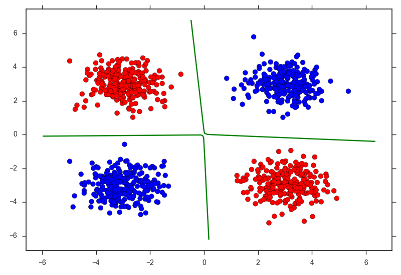
print("Accuracy:", metrics.accuracy_score(yte, ypred)) # Accuracy: 1.0決定境界を図示すると以下のようになりました.
xx, yy = np.meshgrid(
    np.linspace(np.min(X[:,0])-1.0, np.max(X[:,0])+1.0, 100),
    np.linspace(np.min(X[:,1])-1.0, np.max(X[:,1])+1.0, 100)
)

Z = F.softmax(model.predictor(np.float32(np.c_[xx.ravel(), yy.ravel()]))).data[:,1]
Z = Z.reshape(xx.shape)

import seaborn as sns
sns.set_style("ticks")
colors = np.array(["r", "b"])
plt.scatter(X[:,0], X[:,1], c=colors[y], s=50)
plt.contour(xx, yy, Z, levels=[0.5], linewidth=3, colors="g")
plt.tight_layout()
plt.show()